Pythons and Unicorns and Hancitor…Oh My! Decoding Binaries Through Emulation

This post is also available in: 日本語 (Japanese)

This blog post is a continuation of my previous post, VB Dropper and Shellcode for Hancitor Reveal New Techniques Behind Uptick, where we analyzed a new Visual Basic (VB) macro dropper and the accompanying shellcode. In the last post, we left off with having successfully identified where the shellcode carved out and decoded a binary from the Microsoft Word document.

Often when analysts are faced with an embedded payload for which they want to write a decoder, they simply re-write the assembly algorithm in their language of choice and process the file. The complexity of these algorithms varies when attempting to translate from machine code to a higher-level language. It can be quite frustrating at times, depending on the amount of coffee you’ve had and complexity of the algorithms.

In this post, I’ll show how we can use an attacker’s own decoding algorithm combined with CPU emulation to decode or decrypt payloads fairly easily by simply reusing the assembly in front of us. Specifically, I’ll be focusing on using the Unicorn Engine module in Python to run the attacker’s decoding functions within an emulated environment to extract our encoded payloads. Our end goal is to identify the command and control (C2) servers being used by the final Hancitor payload by running our Python script against the Microsoft Word document.

Now, you may ask, why even worry about this to begin with? In the last post we just let the program run and the payload was written to disk for easy retrieval, so why bother? The main answer to that is bulk-analysis automation. If we can write a program that we can point at a directory full of documents, then we can quickly extract embedded payloads for C2 extraction and parsing to form a more holistic view of what we’re dealing with. An example of such bulk analysis was witnessed earlier this year in July when we looked at a large sample set of LuminosityLink malware samples.

Decoding Routines

As a reminder, in the last blog post we were working with the following sample:

03aef51be133425a0e5978ab2529890854ecf1b98a7cf8289c142a62de7acd1a

We’ll continue where we left off after identifying the decoding routine, as seen in figure 1. The function at loc_B92 added 0x3 to each byte and uses 0x13 to XOR the result. Once every byte in the embedded binary has been processed, it pushes the location of the embedded binary to the stack and calls function sub_827.

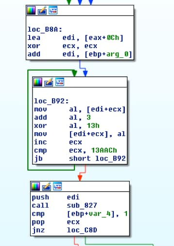
Figure 1 Start of decoding routine

Without going too far into detail on the decoding routine, know that there are five parts to it, and that each one manipulates the bytes in some way before the overall function ends and our payload is decoded.

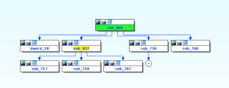
Figure 2 Proximity view of decoding functions in IDA

What we’re effectively going to do is copy the bytes from sub_8A6, sub_827, sub_7E7, sub_7CA, and sub_7D7. These are the core functions that handle all of the decoding. In addition to this, we’ll need our embedded payload, which can be located in the Word document through the magic header of “POLA” as discussed in the previous blog.

Once we have the copied bytes, we’ll setup our emulation environment, adjust our assembly, and run our own shellcode to retrieve the payload. In the context of this blog, I’m just going to refer to the x86 instructions as shellcode to keep things straightforward.

Starting with offset 0xB92, we’ll copy the bytes for the two blocks, ending just after our call since the payload will be decoded by that point.

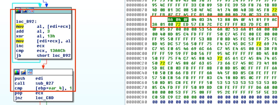
Figure 3 Decoding function and associated bytes

Next we’ll copy the bytes from sub_827, which are all of the bytes from offset 0x827 to 0x8A5.

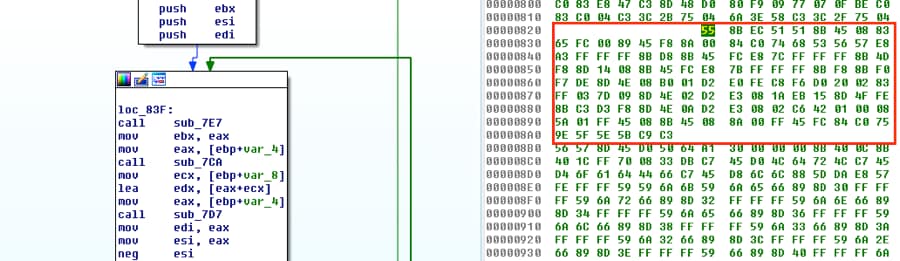
Figure 4 Additional decoding functions and associated bytes

Last, we’ll collect the bytes from the three smaller functions. If you note their location, you can see they are contiguous. Keeping the bytes in order is convenient but not necessary. If they don’t line up, you’ll simply need to adjust the operands for the calls or jumps so that they go where they should.

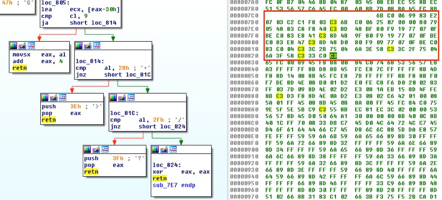
Figure 5 Additional decoding functions and associated bytes

Once all of the bytes have been saved, we can write them to a file and open it up in a disassembler to see what issues we need to correct, if any.

Looking at our shellcode, only one major issue appears, which is the initial call to the decoding function being at a different address.

Figure 6 Broken call within shellcode

As we want to call to our previous function sub_827, which is at the end of our shellcode, we can adjust this call to point to the start of that function. Looking at our code in a hex editor, the start of the function is exactly 97 bytes (0x61) into our shellcode, so we can change the instruction 0xE87CFCFFFF to 0xE861000000.

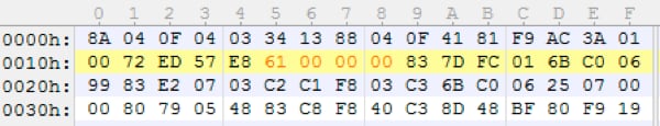
Figure 7 Correcting the previously broken call

Next, we can validate our change worked as expected within the disassembler and that our functions are now all correctly linked.

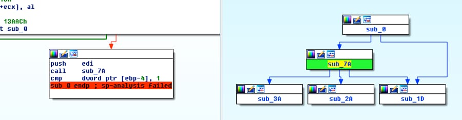
Figure 8 Validating correction of call

Embedded Payload

We know that our embedded payload address is located on the EDI register that gets pushed onto the stack through our previous dynamic analysis. For the initial validation of this method, we’ll go ahead and manually copy the bytes, starting with the magic header of “POLA” and a size of 0x13AAAC bytes, to our Python script. At the end of the blog, I’ll include a full script that will automatically extract this binary from the Word Document.

Enter the Unicorn

As we now have all of the data we need to decode the binary, the last step for this part is to build the emulation environment for our code to run on. To accomplish this, I’ll use the open-source Unicorn Engine.

The first thing we’ll want to do is assign the address space we’ll be working within, along with initializing Unicorn for the architecture we want to emulate (x86), and map some memory to use. Next we’ll write our shellcode and encoded binary to our memory space and initialize some values. Finally, we’ll output the decrypted data to STDOUT.

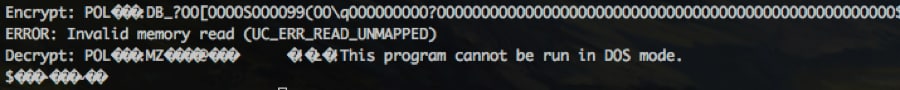
Figure 9 Successful decoding

Success! We can write that section of memory to a file and see what we have.

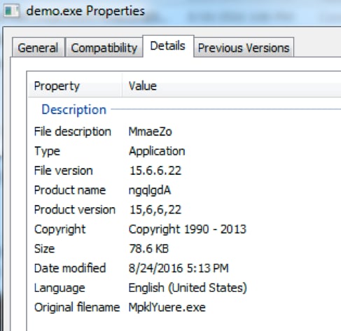
Figure 10 Decoded binary properties

Unfortunately we find ourselves with a packed binary that may have our actual Hancitor sample, so we’ll need to try and decode yet another payload.

Attack of the Binaries

This binary has a fair amount of functions and code, but very early on we see the binary lookup the address for the same API we discussed in our earlier blog post, RtlMoveMemory(), and then copy what we presume is our encoded payload.

Figure 11 RtlMoveMemory() being called

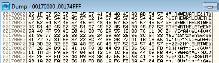
Figure 12 Encoded payload

Continuing to debug the program, just three instructions later it returns to what looks like our next decoding routine.

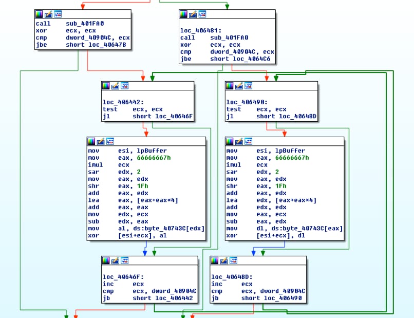
Figure 13 Decoding function

Letting these blocks complete a few times validates we’re in the right spot, as we quickly identify the MZ executable header.

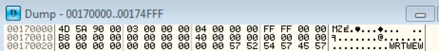
Figure 14 Validation of decoding

We’ve now found the location of the encoded binary, due to RtlMoveMemory(), and the location of our function that we need to emulate.

Function Copying

Analyzing this function, it’s much less complex than the last one, but takes a different approach of iterating over a 12-byte key, located at 0x40743C in our example, and using it to XOR the encoded payload.

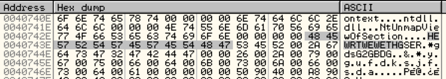
Figure 15 12-byte XOR key

We’ll follow the same methodology as previous to add it into our program.

Starting at loc_406442, we’ll copy all of the bytes for the three blocks in the picture below, which is the decoding loop.

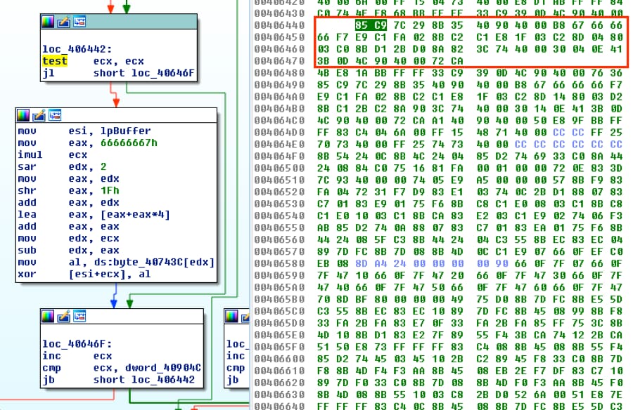
Figure 16 Decoding loop and associated bytes

Next we’ll copy the XOR key and encoded payload into our script and build a test file so that it follows the following order of operation:

shellcode -> key -> payload

Looking at the code in the disassembler, we can tell there are a few values we’ll have to prep before we can make this code run in our emulated environment. Specifically, we’ll need to edit two MOV instructions and a CMP instruction that reference locations that don’t exist in our code.

Based on our dynamic analysis, we know that the lpBuffer is a pointer to the address of the encoded payload, so we can change this instruction to move the starting location, where our payload will reside, into the ESI register. The current instruction is referencing an address in the data segment that holds the address to the payload. We’ll replace it with an immediate MOV instruction by changing 0x8B3540904000 to 0xBE42000190, where 0x100042 is the start of our buffer. Since we changed the opcode, the length of our new instruction was one byte short and I padded it with a 0x90 – NOP to keep everything aligned.

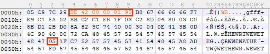
Figure 17 Change location of payload

The first MOV is for our encoded payload, the second MOV is for our XOR key. The second MOV uses a different opcode that plays more favorably to our needs, so we’ll simply change the existing address to the location of the key by modifying 0x8A823C744000 to a value of 0x8A8236000001.

Figure 18 Change location of the XOR key

The final item to change is the compare instruction. Based off dynamic analysis, we know it’s looking for the value 0x5000, so we’ll change the opcode to support an immediate operand and modify 0x3B0D4C904000 to a value of 0x81F900500000.

Figure 19 Hard-set compare value

Emulation

To set up our environment for this sample, the only value we need to worry about is EDX, which needs to be a pointer to our encoded payload, and gets moved into the EAX register during the loop. Similar to before, we’ll setup our address space, define the architecture, map memory, and configure some initial register values.

This yields the following result:

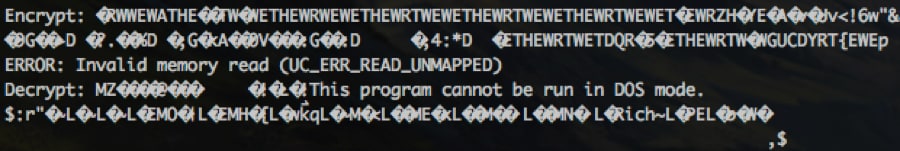
Figure 20 Decrypted payload after running Python script

If we take a look at this binary and peer at the strings, we can see that we’re finally at the end of the road.

Figure 21 Hancitor C2 URLs, external IP check, and Google remote check

To recap the process:

• Started with a Microsoft Word document
• Extracted base64 encoded shellcode
• Extracted encoded payload
• Emulated decoding function from shellcode to decode payload (binary)
• Extracted XOR key from new binary
• Extracted next encoded payload from new binary
• Emulated decoding function from new binary to decode Hancitor (binary)

Our last step is to put everything together into a nice package that we can use to scan thousands of Microsoft Word documents containing Hancitor and identify all of the C2 communications. Here’s a link to the Hancitor decoder script we created.

For the purpose of this test, I took a small sample set of 10,000 unique Microsoft Word documents that were first seen on August 15, 2016 and observed by Palo Alto Networks WildFire as creating a process with a name of “WinHost32.exe”. This, coupled with a few other criteria, gives me a corpus of testing samples that we know will be Hancitor and that I can run this script against.

Analysis

The results were fairly unimpressive, however you win some and you lose some. It still provides some interesting observations.

For our sample set, there were only 3 C2 URLs across all 8,851 Hancitor payloads we successfully decoded:

Looking at the stage 1 payloads, we decoded 9,967, which is almost the entire set. Reviewing the metadata for the PE files, 8,851 exhibited the following characteristics, which are included in a YARA rule at the end of this document.

CompanyName: 'SynapticosSoft, Corporation.'
OriginalFilename: 'MpklYuere.exe'
ProductName: 'ngqlgdA'

Additionally, we identified three XOR keys being used in stage 1:

After correlating the data, each of the keys corresponded to a different stage 2 dropper and our script was designed to target and decoded the most heavily used. General observations for the other two decoders are that the one with key 0xE uses the same XOR key for the second stage Hancitor payload “HEWRTWEWETHG” and would likely be straightforward to add to the decoding script. The 1,103 other files with key 0x14 were identified as Nullsoft Installers.

For the 8,851 that successfully decoded their stage 2 payload, I did not note any PE’s with any file information; however, a YARA rule is included which matches them all. The last thing I’ll mention regarding the stage 2 files is the different file sizes.

This data is pulled from the variable in our shellcode and we can see that there is a slight file size variation in the 13 that used the XOR key 0xE, which might imply slightly modified payloads.

Conclusion

Hopefully this was an educational demonstration using the extremely powerful Unicorn Engine to build a practical malware decoder. These techniques can be applied to many different samples of malware and can free you up from the more tedious process of figuring out how to program a slew of bitwise interactions and focus more on analysis and countermeasures.

Indicators

At the following GitHub repository, you will find 3 YARA rules, listed below, which can be used to detect the various pieces described throughout these two blogs, and the script that was built throughout this blog for decoding Hancitor.

hancitor_dropper.yara – Detect Microsoft Word document dropper
hancitor_stage1.yara – Detect first PE dropper
hancitor_payload.yara – Detect Hancitor malware payload